Alignment correction

After the alignment is made, it normally still is not optimal for modelling purposes. Sequence alignment programs are optimised for the detection of evolutionary relations. This is not always the same as a structural relation. The best example is the deletion of a loop as shown in figure 7.

 1   2   3   4   5   6   7   8   9   10  11  12  13  14
PHE ASP ILE CYS ARG LEU PRO GLY SER ALA GLU ALA VAL CYS (green in fig 8)
PHE ASN VAL CYS ARG THR PRO --- --- --- GLU ALA ILE CYS (red in fig 8)
PHE ASN VAL CYS ARG --- --- --- THR PRO GLU ALA ILE CYS (blue in fig 8)

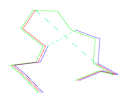
The top line in figure 7 is the template sequence, the bottom two lines are two alternative alignments of the model sequence. Everyone would expect the middle line to be correct, because the alignment of the PROs at position 7 give such a strong signal. In figure 8, you see a Ca trace of three loops. The template is given as A. The middle alignment, corresponding to the red Ca trace, leaves a gap of about 10 Angstrom. However, if we use the bottom alignment, we get situation C which has a gap of only about 5 Angstrom. The normal Ca - Ca distance is 3.8 Angstrom. A 5 Angstrom Ca - Ca distance therefor is actually only a 1.2 Angstrom gap, and that can be closed easily with only minimal atomic displacements.

Figure 8. The Ca traces resulting from the alignment in figure 7. Green: template. Red: middle alignment from figure 7. Blue: bottom alignment from figure 7.

Figure 8 again. The same figure as above, but now with all residues indicated...

Another example of alignment problems is the alignment of the haemoglobin alpha and beta chains. This alignment will (almost independent of the alignment program used) look like (figure 9):

        1       5        10        15        20        25        30
        - V L S P A D K T N V K A A W G K V G A H A G E Y G A E A L
        V H L T P E E K S A V T A L W G K V - - N V D E V G G E A L

       31      35        40        45        50        55        60
        E R M F L S F P T T K T Y F P H F - D L S H - - - - - G S A
        G R L L V V Y P W T Q R F F E S F G D L S T P D A V M G N P

       61      65        70        75        80        85        90
        Q V K G H G K K V A D A L T N A V A H V D D M P N A L S A L
        K V K A H G K K V L G A F S D G L A H L D N L K G T F A T L

       91      95       100       105       110       115       120
        S D L H A H K L R V D P V N F K L L S H C L L V T L A A H L
        S E L H C D K L H V D P E N F R L L G N V L V C V L A H H F

      121     125       130       135       140       145       
        P A E F T P A V H A S L D K F L A S V S T V L T S K Y R 
        G K E F T P P V Q A A Y Q K V V A G V A N A L A H K Y H 

Around residue 50 we see a strong identical triplet: DLS. However, if you study the superposed structures of these two chains, you will see that Asp 49 of the a-chain should be aligned with Gly 48 from the b- chain.

Figure 10 shows the Ca traces of the a and the b chain superposed. The side-chains of His 52 from the a-chain and Met 57 from the b-chain are shown too. Not only do these two sidechains occupy approximately the same space, but an antroposophical analysis makes clear that they both have the same function: they glue the otherwise rather detached loop around residue 50 to the core of the protein. The histidine in the A subunit does this via a saltbridge with a glutamic acid (which is also indicated in figure 10); the methionine in the B subunit does it via hydrophobic contacts, mainly with the bacbone of a nearby helix.

It should be stressed that the alignment errors shown here are not errors in the alignment programs, but errors made by our gambler and our modeller. The alignment programs are optimised to detect evolutionary relationships between proteins, and for that purpose they try to determine what actually happened at the nucleic acid level. Although this can not be seen separately from what happened at the protein level, it is clearly a different thing. Thus, sequence alignments that are perfect in an evolutionary sence, are not always perfect for homology modelling purposes.

Placing new side chains in the structure

When we study the rotamers of residues that are conserved in different proteins with known (similar) three dimensional structure we observe in more than 90% of all cases similar c1 angles. It will be shown below that modellers do not reach that percentage upon modelling, and therefore the advise given by our gambling friend ³Donıt touch the conserved ones, your odds are better that way² is followed by most modellers. The problem of placing side chains is thus reduced to concentrating on those residues that are not conserved in the sequence.

In case of high sequence homology between the structure and the model the main problem lies just in the replacement of a few side chains. Often this can be done by hand [11,91,92,103], using an interactive molecular graphics package. Alternatively, one tries to find examples of residues in a similar environment [93] in the database of known structures. The problems here are how to define similar environments, and how to extract the information quickly from the database of known structures. In practice, similar environments for residues have most often been defined as having the same secondary structure (a-helix, b- strand or loop). In this review we will emphasize the power of position specific rotamer distributions.

The problem of side chain modelling can be divided in two sub- problems: 1) finding potentially good rotamers, and 2) determining the best one among the candidates.

Until recently side chain conformations were normally selected using standard rotamer libraries [94-96], and a variety of procedures, ranging from manual adaptation to complicated schemes involving energy calculations or Monte Carlo procedures combined with energy calculations, have been used to get rid of Van der Waals clashes, and to find the global optimum among all rotamer combinations [97-100]. Recently, however, several studies indicated that the use of standard rotamer libraries is far from optimal because a large fraction of the information needed to determine the side chain rotamer is contained in the local backbone [100,103-106]. The study by De Filippis et al., [103] has the most direct applicability to statistics based homology modelling and will therefore briefly be summarised.

Position specific rotamers

A single mutation in a protein can dramatically influence its stability or function. However, large structural changes as a result of one single mutation are rare. Generally, the overall structure of proteins does not change upon introduction of a point mutation. If a mutated amino acid does not fit well into its environment, conformational adaptations are made mainly by the mutated residue, to a lesser extent by its entire secondary structure element, and rarely by its three dimensional contact partners. Calculation or even estimates of free energy changes are insufficiently accurate to be used as a routine tool for predicting structural changes. On the other hand, empirical methods based on a variety of approaches work quite well for some purposes [e.g. 108-111]. A reliable and general theory of side chain rotamers, however, does not yet exist.

De Filippis et al., therefore consulted our 21 player and developed a statistical method for predicting structural changes that is based on searches in the database of 3D structure. Given a residue to be mutated, they search the database for residues with a similar environment and then assess which rotamers in the database are statistically preferred and sterically admissible in the current structure. Using simple rules based on this scheme the local structural environment of a point mutation can be predicted correctly in the majority of all cases. They analysed almost 100 point mutated proteins with know wild type and mutant structure.

For every mutant, a position-specific rotamer analysis was performed. This technique has been described in detail elsewhere [112- 114]. Briefly, a rotamer distribution at a certain position is determined by extracting from a database of non-redundant protein structures [115,116] all suitable fragments of length 5 or 7 residues (7 in helix and strand, 5 in case of irregular local backbone). Suitable fragments are those that have a local backbone conformation similar to the one around the evaluated position, and have the same residue type at the central position. In these analyses, the RMS deviation of the alpha carbon positions between the structure and the database fragment was kept below 0.5 Angstrom. The rotamer distributions were then used to answer the following questions:

• What are the differences between the rotamer of the residue mutated by protein engineering and the position specific rotamer distribution obtained from the database of natural proteins?
• Which set of rules would have allowed us to predict the structure of the mutated residue correctly?

1. There is only one way of placing the residue without atomic clashes. In all 4 examples in this class they found just one rotamer that leaves the rest of the molecule unaltered and this is the observed rotamer.
2. The conformation of the mutated residue corresponds to the most populated position-specific rotamer. This occurs in approximately 50% of all cases.
3. The most populated rotamer would lead to atomic clashes and the conformation of the mutated residue corresponds to the second most populated rotamer (4 examples).
4. Neither the most populated, nor the second most populated rotamer fits, and the conformation of the mutated residue is very close to the most populated rotamer (2 examples found, both deviate about 20š from the optimal c1). Never did they observe that the third, i.e., least populated rotamer was selected.
5. The c1 of the mutated residue corresponds to the most populated rotamer, but the c2 or c3 angle is rotated away from the optimal position-specific rotamer distribution to optimise hydrogen bonding. This is observed in almost 15% of all cases (10 examples).
6. There is no preferred position-specific rotamer, or there are insufficient examples in the database, but analysis of potential hydrogen bonds leads to one clear possibility for the structure. This occurs in 7% of all cases (4 examples). Although in these cases it is possible to fix the charged end of the side-chain in the proper position, it is often difficult to accurately predict the correct conformation of the hydrophobic part of the side-chain.

These six observed classes were converted into a set of rules (See figure 11). Assuming that their dataset is representative of the universe of mutated residues, then this scheme allows to correctly predict the local structures of at least 85% of all mutated residues. The actual predictive ability on proteins not studied here may, of course, be lower.

Of the six rules, the first three are the most clear-cut, i.e. have a high prediction accuracy. These rules cover about 60% of all cases. In all other cases, the prediction accuracy is lower on average. Reassuringly, however, there is a qualitative correlation between correct prediction and the quality of fit of database fragments on the actual backbone, the number of observed database fragments and the sharpness of the c1 distribution of the central residues in these fragments.

They conclude with the notion that not all conformational changes resulting from point mutations can be predicted correctly with the techniques available to date. Examples of changes difficult to predict are large domain motions or local structure adaptations induced by co- factor binding.