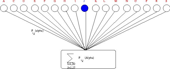
Description of the GOR-III
algorithm. Probabilities (Pij) is summed ovver all
residues in a window. All these together are used to predict the
secondary structure of one central residue (residue J marked in
blue in this figure).
As we all know proteins consist of secondary structure elements. The prediction of these elements might help us to understand more about the function of these proteins without determine its three-dimensional structure. Further it has been believed that prediction of secondary structures is a step toward the prediction of the three-dimensional structure of a protein. Lately it has also been shown that secondary structure predictions can be included in threading methods to help the detection of distantly related proteins.
A long time ago experiments showed that some synthetic polypeptides had different intrinsic ability to form different types of secondary structure. This lead to the assumption that secondary structure was (partly) formed by the local sequence. However, it has also been noticed that long segments (up to 11 amino-acids) of identical sequences might form different secondary structures, i.e. the secondary structure is not only decided by local factors.
Today almost all secondary structure prediction methods are based on the propensities for amino acid residues to form beta-strands, helices or turns. These propensities have been derived from studies of the conformation of small peptides in solution, or from statistical analysis of the occurrence of certain residues in the various types of secondary structure in known structures. Most secondary structure methods only take into local factors, and do completely ignore long range interactions.
It should be noted that most secondary structures predictions only predict three (or sometimes four) different secondary structures, while in proteins several others exist. Therefore, the prediction of pi-helices and other more rare secondary structure elements can not be performed using the methods described here. Also, the prediction of secondary structures in membrane proteins is better using predictors specifically trained to predict these. These will be described in the membrane section.
The question of how to compare different secondary structure prediction methods is more complex than one might first imagine. Two primary issues are: what statistic(s) should one report and how should a database of proteins with known structure be selected and used? The question of statistics is largely historical. Customarily procedures have been evaluated by the percentage of amino acids whose secondary structure class (usually helix, coil, or sheet) is correctly predicted. This statistic is often referred to as the Q3. Some authors have begun to favor use of a correlation coefficient between predicted and observed secondary structure. This measure avoids the problem of rewarding over prediction of more common secondary structure classes in the database, but is much less intuitive for the reader to interpret. At this time, most authors report both correlation coefficients and Q3s. However, Q3 is still the most common measure.
The choice of database is also complex. To obtain reliable statistics at least ~120 proteins, none of which are homologous to a protein used in for the training. However, to completely exclude homology is quite difficult. Inclusion of the protein of interest in the parameter optimization can artificially inflate the performance statistics (e.g. an improvement in Q3 for the GOR method (Garnier et al., 1996 ) of 5.3%, or 64.4 % to 69.7% accuracy (from Holley and Karplus, 1991). Since the goal is to accurately model secondary structures of proteins with unknown tertiary structures, this inflation is clearly a failure to accurately assess prediction accuracy.
1974 Chou and Fasman propose a statistical method based on the propensities of amino acids to adopt secondary structures based on the observation of their location in 15 protein structures determined by X-ray diffraction. These statistics derive from the particular stereochemical and physicochemical properties of the amino acids. These statistics have been refined over the years by a number of authors (including Chou and Fasman themselves) using a larger set of proteins. On a larger set of 62 proteins the base method reports a success rate of about 50%. From these structures they calculated the probability for each residue to be in a certain secondary structure type. The residues where then classified into different groups, for instance Glu, Met Ala and Leu where classified as strong Helix formers, while Val, Ile and Tyr where strong sheet-formers. The following classes were created:
From listing of these properties the prediction was done in a semi-manual fashion. By initiating a helix in a region with strong helix formers and using a similar set of rules it is possible to obtain a prediction of the secondary structure.
When more structures were known, it was possible to calculate a more accurate statistics for the secondary structure preferences for the different amino acids. Chou and Fasman introduced the Pij values in 1978. These values describe the probabality to find a certain amino acid in a type of secondary structure. The table of numbers is as follows:
Name           P(H)   P(E)   P(turn)    f(i)    f(i+1)  f(i+2)  f(i+3)

Alanine        142     83       66      0.06    0.076   0.035   0.058
Arginine        98     93       95      0.070   0.106   0.099   0.085
Aspartic Acid  101     54      146      0.147   0.110   0.179   0.081
Asparagine      67     89      156      0.161   0.083   0.191   0.091
Cysteine        70    119      119      0.149   0.050   0.117   0.128
Glutamic Acid  151    037       74      0.056   0.060   0.077   0.064
Glutamine      111    110       98      0.074   0.098   0.037   0.098
Glycine         57     75      156      0.102   0.085   0.190   0.152
Histidine      100     87       95      0.140   0.047   0.093   0.054
Isoleucine     108    160       47      0.043   0.034   0.013   0.056
Leucine        121    130       59      0.061   0.025   0.036   0.070
Lysine         114     74      101      0.055   0.115   0.072   0.095
Methionine     145    105       60      0.068   0.082   0.014   0.055
Phenylalanine  113    138       60      0.059   0.041   0.065   0.065
Proline         57     55      152      0.102   0.301   0.034   0.068
Serine          77     75      143      0.120   0.139   0.125   0.106
Threonine       83    119       96      0.086   0.108   0.065   0.079
Tryptophan     108    137       96      0.077   0.013   0.064   0.167
Tyrosine        69    147      114      0.082   0.065   0.114   0.125
Valine         106    170       50      0.062   0.048   0.028   0.053
The actual algorithm contains a few simple steps:
p(t) = f(j)f(j+1)f(j+2)f(j+3)
where the f(j+1) value for the j+1 residue is used, the f(j+2) value for the j+2 residue is used and the f(j+3) value for the j+3 residue is used. If: (1) p(t) > 0.000075; (2) the average value for P(turn) > 1.00 in the tetrapeptide; and (3) the averages for the tetrapeptide obey the inequality P(alpha-helix) < P(turn) > P(beta-sheet), then a beta-turn is predicted at that location.
The simple Chou-Fasman prediction method can be performed with a pencil and a piece of paper, although a programmed version is normally used.This method performed quite well (about 60% accuracy)
Other groups (Lim, Garnier J, Osguthorpe DJ, Robson B) developed other secondary structure prediction methods based on similar ideas as Chou and Fasman. None of these method reached over 60% accuracy in independent tests.
The earlier methods for secondary structure predictions do only take into account the information for one amino acid at a time. However, it can be assumed that if a particular amino acid is surrounded with residues that prefer to be in a helix it is likely in a helix even if its helical preference is quite low. Further it was observed that specific residues are more likely to start (or end) secondary structure elements, e.g. in helix capping. Therefore it might be advantageous to use information not only from a single reside, but instead from a window of residues.
A somewhat more sophisticated method is the Garnier-Osguthorpe-Robson (GOR III) method. In this method, an attempt has been made to include information about a slightly longer segment of the polypeptide chain. In stead of considering propensities for a single residue, position-dependent propensities for helix, sheet and turn has been calculated for all residue types. The GOR III method is also significantly cleaner and easier to code than earlier methods. It is based on the same Pij values as in the second Chou Fasman method. The performance of GOR-III is about 63% Q3.
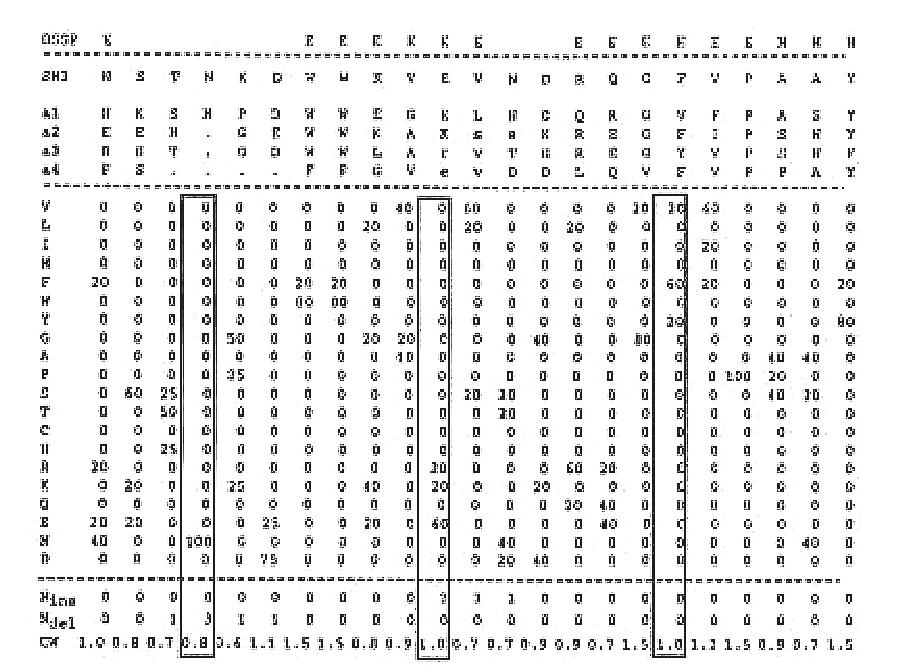
The theory began as essentially a more rigorous method than calculating Chou-Fasman-like propensities for calculating the probability of a given amino acid assuming a given secondary structure element. The bridge to this probability is a function called the information: I(S , R) = log (fS,RN/fRfS). In this equation, fS,R is the frequency of amino acid R in secondary structure S in the database, N is the number of amino acids in the database, and fR and fS are the frequencies of R and S in the database, respectively. It can be shown that the secondary structure with the highest I is the most likely one for a given amino acid. Generally, the value of I(S,R) is not used; rather a value termed I(DS,R) which is the difference in I between a given S and the sum of all other possible Ss. Also, since the amino acids which neighbor a given residue are also a source of information about its conformation, they too are used. The GOR-III algorithm can be outlined as follows:
Description of the GOR-III
algorithm. Probabilities (Pij) is summed ovver all
residues in a window. All these together are used to predict the
secondary structure of one central residue (residue J marked in
blue in this figure).
This predicted will therefore be influenced not only by the actual residue at that position, but also to some extent by other neighboring residues. The propensity tables will to some extent reflect the fact that prolines can be found in the C-terminal end of helices, but are very unlikely in the N-terminal end. They will also reflect that positively charged residues are more often found in the C-terminal end of helices and that negatively charged residues are found in the N-terminal end. The GOR method is well suited for programming and has been a standard method for many years.
The nearest neighbor method of secondary structure prediction has also been called memory-based, exemplar-based, or the homologous method. The method is performed by finding some number of the closest sequences (from a database of proteins with known structure) to a subsquence defined by a window around the amino acid of interest. Using the known secondary structures of the aligned sequences (generally weighted by their similarity to the target sequence) a secondary structure prediction is made. Though the method is simple to describe, a number of undefined parameters in the above description allow the method to be applied in a wide range of ways, with a similarly wide range of results. Sequences are chosen based on their similarity, but in what fashion is similarity defined? What size window of sequence should be examined? How many close sequences should be selected? Several methods, all nearest neighbor in approach, but each using a different set of these parameters have been created.
The nearest neighbor method relies on selecting the closest subsequences to a window around the amino acid which is being predicted. Of course, this can be done in a number of ways. Zhang, et al. use a distance measure reminiscent of the probabilities used in the information theory of the GOR method (above). Salomov and Solovyev's SSPAL method is significantly more successful. The first difference is the use of alignments of varying size, which may contain gaps. The authors claim that this allows the algorithm to access information which normal nearest neighbor methods may sacrifice. One can imagine how this might be the case for Zhang, et al.'s method. Imagine an alignment of the sort:
HHH-EE
HHHHEE
where H will be taken to mean a residue with strong helical potential and A a strong beta potential. Without allowing for gapped alignment, the score of this alignment will drop, perhaps significantly.
A second difference in the alignment is the use of a new scoring scheme, which uses both sequence similarity akin to that used by Zhang et al., and a 3D-1D score. This scoring method creates a distance matrix from the frequencies with which each amino acid appears in a given, defined chemical environment, e.g. "buried and partially polar." When a potential alignment is considered, part of the score dervies from the propensity of the amino acid being aligned to be in the (known) environment of the sequence in the database. Use of this type of scoring scheme generates a 4% improvement in accuracy (Yi and Lander, 1993).
Third, the first step in the algorithm is the reduction of the database for a given alignment from ca. 120 to the 90 proteins with closest pairwise Chou Fasman parameters. This method was previously explored in a method which attained a Q3 of only 67.6%. Thus, this step likely unresponsible for about 4% of the improvement in accuracy.
Last, the authors of SSPAL use more alignments (50 vs. 25 for Zhang, et al.) to generate their prediction. This likely has little impact on the quality of their prediction, since use of 20 or 30 alignments both yield ~71% accuracy, still far ahead of the Zhang algorithm.
As noted above, this method might outperforms information theory, likely due to its ability to access third and higher order interactions (rather than only pairwise) and outside the window used by GOR.
After the introduction of GOR III in 1987, several methods tried to improve the performance using similar approaches. These methods included neural networks, nearest neighboring methods and hidden Markov Models. None of these methods reached a higher accuracy then about 65% for a well created test set. Therefore, it was assumed for a long time that it was not possible to obtain higher accuracy without taking into account long-range interactions. Even if the prediction accuracy was about 65% it was hard to decide the exact number of secondary structure elements from a predictions as many predited structures often was to short:. Further, the prediction accuracy of beta-sheets was significantly lower than 65%.
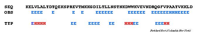
Example of prediction in the early 1990s
At the same time several groups made manual secondary structure predictions that reached a higher accuracy than 65%. Obviously, people started toexamine what was the manual knowledge that could be used to improve the predictions but was not already included. It was noted that one of the most important factors where the inclusion of evolutionary information.
Since 1993 a number of methods that show significantly better results than the above methods have been developed. The improvement comes from using multiple aligned sequences for the prediction. The pattern of substitutions in homologous proteins contains information about features that are of importance for the fold of a protein. If the protein of interest can be aligned with homologous sequences, the consensus sequence will give improved accuracy for the prediction.
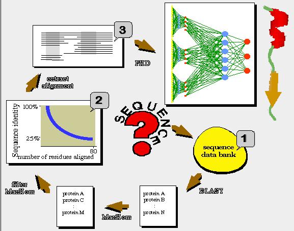
Example of input to PhD
The first program to use evolutionary information was PhD, which is based on a two-layered feed-forward neural network . The accuracy for this on aligned homologous sequences was the first program to reach over 70%. In the neural network, aligned homologous sequences of known structures are used to "train" the network, which then can be used to predict the secondary structure of the aligned sequences of the unknown protein.
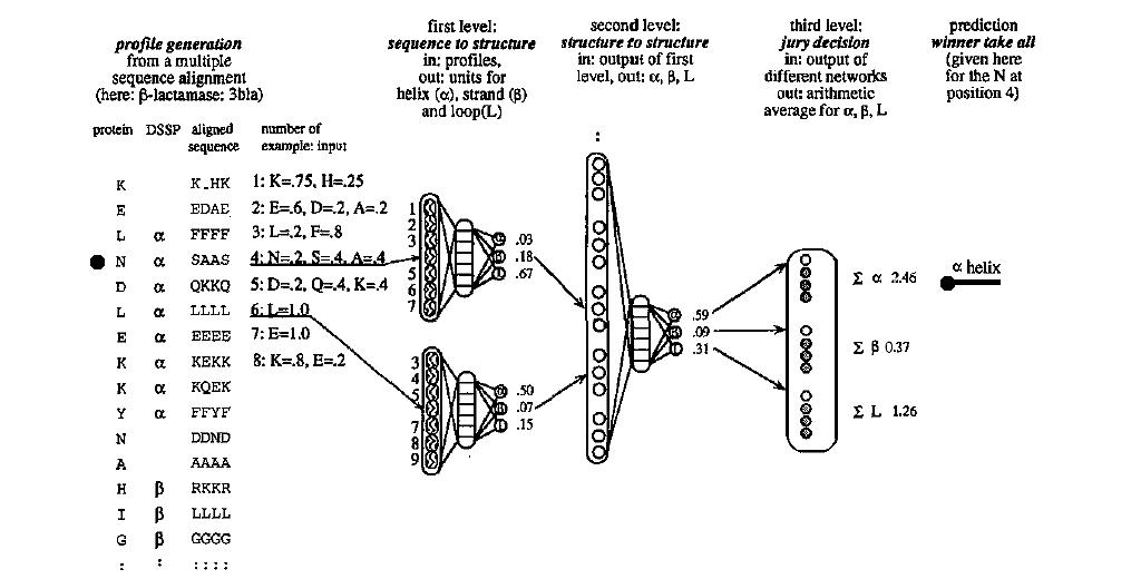
Description of the PhD
method. PhD starts from a multiple sequence alignment and then
uses three layers of networks to predict the secondary structure
of the central residue.
One important aspect when creating PhD was that a carefully created set of non-related proteins was used. The neural networks in PHD (see picture) can be described to function as follows:
The main improvement over the other methods described above is due to the aligned sequences. For example, positions where insertions and deletions have occurred are most likely to correspond to loop regions. The main improvement in PhD can be summarized as follows:
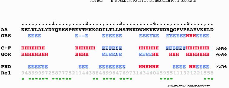
Example of prediction using PhD
Since the introduction of PhD, many methods using evolutionary information has been introduced. The performance of all these methods are quite similar. However, there has been an incremental improvements in secondary structure predictions. The current state of the art methods perform readily over 75% Q3 accuracy. Some of the this improvements can be attributed to:
However, also minor changes in the algorithms has contributed to the improvement. Today one of the best, and easiest to use, programs is psipred that use profiles as their input to the a neural network.
It seems as if it is possible to reach close to 80% accuracy using todays methods and more sequence information. To reach higher accuracy it might be necessary to define secondary structures better as well as take long-range interactions into account.
Obviously similar techniques as described here can be use to predict other type of local features in a protein. For instance the PhD program is nowadays also trained to predict the exposed surface area of each protein. In a simple definition of inside/outside it is possible to obtain more than 75% accuracy in this type of predictions.