So far we have concluded that it might be useful to obtain an alignment of two sequences. If you have enough time it is possible to make a manual alignment, by for instance using a dotplot analysis. Still there are many examples where a trained bioinformatician might make a better alignment than can be obtained by automatic methods, especially for multiple sequence alignments. However, for most non-trained bioinformaticians or for large scale analysis it is absolutely necessary to use automatic methods to obtain alignments. The question is then how do we obtain the best possible alignment.
To find an algorithm that can be used to obtain the best possible alignment, we need to define what is the best possible alignment. A convenient way to do this is to assign a score to the alignment of each type of residue with the alignment of each other type of residue, and also include some scores for gaps. This type of scoring tables are often called substitutions matrixes and is described elsewhere. If this definition of the best alignment method is used , it is possible to use a technique called dynamic programming to find the best possible alignment.
Dynamic programming is one of the most frequently used computer algorithms in bioinformatics. It is used in most sequence search protocols as well in most alignment problems. Often DP is used to find the "best" alignment between two strings (i.e. DNA or protein sequences). However, to explain how dynamic programming works we will use a simpler problem. The problem to detect the longest common sub-sequence between two strings. For you who already know how sequence alignments work this could be seen as a local alignment problem where we do not allow any mismatches and where we use an identity matrix and no gap penalty.
Dynamic programming solves problems by combining the solutions into sub-problems. Dynamic programming can be used when a problem can be divided into sub-problems and when these sub-problems are not independent, i.e. when sub-problems share sub-sub-problems.
DP is most frequently used to optimization problems, for instance to find the best score when aligning two sequences. Each solution produce a certain score and we want to produce the optimal solution, i.e. the solution with the highest (or lowest) score.
DP algorithms can be divided into 4 steps:
Step 4 can be omitted if only the value and not the exact details are needed. This can for instance be used when searching a database, where we are not interested in the alignment but only in the score for a particular match.
To be able to apply DP to a problem there are some criterias that has to be filled. These are: optimal sub-structure and overlapping sub-problems.
A problem exhibit an optimal sub-structure of an optimal solution to the problem contains within it optimal solutions to the sub-problems. In the example of sequence alignments this means that if the problem could be solved with DP it is necessary that the optimal alignment of residues 1 to N includes the optimal alignment of residues 1 to K, where K is less than N.
The second requirement for the use of DP to a problem is that the sub-problems be so that a recursive algorithm for the problem solves the same sub-problems over and over, rather than always generating new sub-problems. When a recursive algorithm revisits the same problem over and over again the DP algorithm typically solves the sub-problem once and then stores the results in a table.
In sequence alignments it is necessary that the score for aligning a certain residue with a another residue is known at the time of the comparisons between these residues. If this is not the case the overlapping sub-problem necessity is broken. One such example is in threading when the score of aligning two residues are dependent on the alignment of other residues, i.e. a new sub-problem is generated all the time. It has been shown that this problem is NP-complete (Lathrop, 1994 Prot. Eng).
Probably the best way to get a better understanding of DP is to study an example. We have chosen the example to find the Longest Common Sub-sequence, or the LCS problem.
In the LCS we find the largest common sub-sequence between two different sequences. A sub-sequence of a given sequence is just a part of this sequence (or the complete sequence). A sequence is just a string of symbols (for instance letters representing amino acids).
In mathematical terms a sequence Z (Z= {z1, z2, z3...., zk}) is a subsequence of X (X= {x1, x2, x3...., xk}) if there exists a strictly increasing sequence {i1, i2, i3...., ik} of indices X such that for all j=1,2,3....,k we have xij1 = zj. For example, Z={B,C,D,B} is a subsequence of X={A,B,C,B,D,A,B} with the corresponding index sequence {2,3,5,7}
Given two sequences X and Y we say that a sequence Z is a common subsequence of X and Y if Z is a subsequence of both X and Y. For example, if X={A,B,C,B,D,A,B} and Y={B,D,C,A,B,A}, the sequence Z={B,C,A} is a common subsequence of both X and Y. The sequence Z1 is however not the LCS of X and Y. Z1 has the length 3 and it is possible to detect another common subsequence Z2={B,C,B,A} of length 4. The sequence Z2 is however not the only LCS as another sequence Z3={B,D,A,B} also exist.
In the LCS problem we are given two sequences X and Y and we want to find a common subsequence Z of maximum length. As you might have guessed this problem can be solved by dynamic programming. We will follow the procedure suggested above, i.e.:
A brute-force approach to solving the LCS problem is to enumerate all subsequences of X and check each subsequence to see if it is also a subsequence of Y. Each subsequence of X correspond to a subset of indices {1,2,...m} of X. There are 2m subsequence of X, so this approach requires exponential time. An algorithm that needs exponential time grows very fast for longer sequences. For instance a sequence of length 20 only needs about 1 million comparisons (220=1048576) but a sequence of 50 needs 1030 comparisons, which would take a longer time to compute than the existence of the universe.
The LCS problem has an optimal-substructure property. Below we will prove that this is the case. The best choice of sub-problems for LCS corresponds to pairs of prefixes of the two input sequences. Given a sequence X={x1, x2, x3...., xm}, we define the ith prefix of X as Xi={x1, x2, x3...., xi}. For example if X={A,B,C,B,D,A,B}, then X4={A,B,C,B} and X0 is an empty string.
oTheorem 1: Optimal Substructure of an LCS: Let X={x1, x2, x3...., xm} and Y={y1, y2, y3...., yn}, and let Z={z1, z2, z3...., zk} be any LCS of X and Y.
(1) If zk!=xm, then we could append xm=yn to Z to obtain a common subsequence of X and Y of length k+1, contradicting the supposition that Z is a longest common subsequence of X and Y. Thus, we must have zk=xm=yn. Now , the prefix Zk-1 is a common subsequence of Xm-1 and Yn-1 of length k-1. We wish to show that Z is an LCS. Suppose for the purpose of contradiction that there is a common subsequence W of Xm-1 and Yn-1 with length greater than k-1. Then appending xm=yn to W produces a common subsequence of X and Y whose length is greater than k, which is a contradiction.
(2) if zk!=xm then Z is a common subsequence of Xm-1 and Y. If there were a common subsequence W of Xm-1 with a length greater than k, then W would also be a common subsequence of of Xm and Y, contradicting the assumption that Z is an LCS of X and Y.
(3) The proof is identical to the proof of (2).
The theorem above implies that there are either one or two sub-problems to examine when finding an LCS of X and Y. If xm=yn, we must find an LCS of Xm-1 and Yn-1. If we find such an LCS we can just append the two values xm and yn to find an LCS of X and Y. However if xm!=yn we have to solve two sub-problems: finding an LCS of Xm-1 and Y and finding an LCS of X and Yn-1. Whichever of these two LCS's is longer is an LCS of X and Y.
We can readily see the overlapping-sub-problems property in the LCS problem. To find an LCS of X and Y, we may need to find the LCS's of X and Yn-1 and Xm-1 and Y. However each of these sub-problems has the sub-problems of finding the LCS of Xm-1 and Yn-1. Many other sub-problems share subsub-problems.
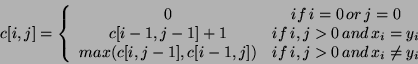
The recursive solution to the LCS problem involves establishing a recurrence for the cost of an optimal solution. Let us define c[i,j] to be the length of an LCS of the sequences Xi and Yi. If either i=0 or j=0, one of the sequence has length 0, so the LCS has length 0. The optimal substructure of the LCS problem gives the recursive formula:
Using the equation above we could easily write a computer program to solve the LCS problem. However that would take exponential amount of time (i.e. it would be very slow for large problems). However, we can also use dynamic programming to solve the problem "bottom-up". This program would only be O(m*n), i.e. the time needed would increase linearly with the length of the two sequences multipled with each other, i.e. the algorithm would be much faster than an algorithm growing exponentially for long sequences.
The procedure takes two sequences X and Y as inputs. It stores the c[i,j] values in a table c[0..m,0..n] whose entries are computed in row-major order. (That is, the first row of c is filled in from left to right, then the second row, and so on.) It also maintains the table b[1..m,1..n] to simplify the construction of an optimal sub-problem solution chosen when computing c[i,j]. The procedure returns the b and c tables; c[m,n] contains the length of an LCS of X and Y. Below is an example of such a code:
m = length[X]
n = length[y]
for i = 1 to m
  c[i,0] = 0
for j = 0 to n
  c[0,j] = 0
for i = 1 to m
  for j = 1 to n
    if (xi = yi)
    then
      c[i,j] = c[i-1,j-1]+1
      b[i,j] = "up-back-arrow (^<-)"
    else if (c[i-1,j] >= c[i,j-1])
      then
        c[i,j] = c[i-1,j]
        b[i,j] = "uparrow (^)"
      else
        c[i,j] = c[i,j-1]
        b[i,j] = "backarrow (<-)"
return c and b
The c table produced by this algorithm for two sequences X={A,B,C,B,D,A,B} and Y={B,D,C,A,B,A} is shown in the table below.
| j | 0 | 1 | 2 | 3 | 4 | 5 | 6 | |
| i | yj | B | D | C | A | B | A | |
| 0 | xj | 0 | 0 | 0 | 0 | 0 | 0 | 0 |
| 1 | A | 0 | ^ 0 | ^ 0 | ^ 0 | ^ 1 | <- 1 | ^<- 1 |
| 2 | B | 0 | ^<- 1 | <- 1 | <- 1 | ^ 1 | ^<- 2 | <- 2 |
| 3 | C | 0 | ^ 1 | ^ 1 | ^<- 2 | <- 2 | ^ 2 | ^ 2 |
| 4 | B | 0 | ^<- 1 | ^ 1 | ^ 2 | ^ 2 | ^<- 3 | <- 3 |
| 5 | D | 0 | ^ 1 | ^<- 2 | ^ 2 | ^ 2 | ^ 3 | ^ 3 |
| 6 | A | 0 | ^ 1 | ^ 2 | ^ 2 | ^<- 3 | ^ 3 | 4 ^<- |
| 7 | B | 0 | ^<- 1 | ^ 2 | ^ 2 | ^ 3 | ^<- 4 | 4 |
The B and C matrix with the LCS {B,C,B,A} is marked in bold:
The b table returned by the program can be used to quickly construct an LCS of X and Y. We begin at b[m,n] and trace through the matrix, following the arrows in the C-matrix. Whenever we encounter an "up-back-arrow" in entry b[i,j], it implies that xi=yi is an element of the LCS. The elemerns of the LCS are encountered in revers order by this method.
If you are lazy and do not want to use a paper and pencil to solve our simple dynamic programming problem. You might be able to use the Dynamic Programming Tabular Computation Demo.